Model Validation & Prediction Assessment in R: Testing Your Models on New Data

Lesson 4

Introduction to Model Validation

You've learned to fit models, compare them statistically, and check diagnostic assumptions. Now comes the ultimate test: How well do your models predict new, unseen data? This lesson teaches validation techniques that separate truly useful models from overfitted ones.

Model validation answers the crucial question: "Will this model work in the real world?" Diagnostic plots tell you if assumptions are met, but only testing on new data reveals true predictive performance.

What You'll Learn

Implement leave-one-out and k-fold cross-validation
Assess prediction accuracy with multiple metrics
Use bootstrap methods for uncertainty quantification
Understand the bias-variance trade-off in model complexity
Distinguish between confidence and prediction intervals
Apply learning curves to assess data sufficiency
Make informed decisions about model deployment

Before You Begin:

Completed modeling, comparison, and diagnostic tutorials
Understanding of overfitting and generalization
Same packages: tidyverse, glmmTMB, broom.mixed
Basic knowledge of sampling and resampling concepts

The Central Challenge: More complex models fit training data better but may perform worse on new data. Validation helps find the sweet spot between underfitting (high bias) and overfitting (high variance).

Step 1

Cross-Validation: The Gold Standard

Cross-validation tests model performance by repeatedly fitting on subsets of data and predicting on held-out observations. This simulates real-world deployment where you must predict new cases.

# Implement Leave-One-Out Cross-Validation
library(tidyverse)
library(glmmTMB)
library(broom.mixed)

data(mtcars)

# Define our competing models from previous lessons
loo_cv <- function(model_formula, data) {
  n <- nrow(data)
  predictions <- numeric(n)
  
  for(i in 1:n) {
    # Fit model without observation i
    train_data <- data[-i, ]
    test_data <- data[i, ]
    
    # Fit model and predict held-out observation
    temp_model <- glmmTMB(model_formula, data = train_data)
    predictions[i] <- predict(temp_model, newdata = test_data)
  }
  
  return(predictions)
}

# Test all our competing models
cv_formulas <- list(
  simple = mpg ~ wt,
  additive = mpg ~ wt + hp,
  interaction = mpg ~ wt * hp,
  complex = mpg ~ wt * hp + cyl
)

# Fit all models to the full dataset for AIC calculation
# Note: These fitted models are needed for AIC comparison and bootstrap methods
models <- list(
  simple = glmmTMB(cv_formulas$simple, data = mtcars),
  additive = glmmTMB(cv_formulas$additive, data = mtcars),
  interaction = glmmTMB(cv_formulas$interaction, data = mtcars),
  complex = glmmTMB(cv_formulas$complex, data = mtcars)
)

# Perform cross-validation for each model
cv_results <- map_dfr(names(cv_formulas), function(model_name) {
  predictions <- loo_cv(cv_formulas[[model_name]], mtcars)
  
  data.frame(
    model = model_name,
    observed = mtcars$mpg,
    predicted = predictions,
    residual = mtcars$mpg - predictions,
    car = rownames(mtcars)
  )
})

# Calculate performance metrics
cv_metrics <- cv_results %>%
  group_by(model) %>%
  summarise(
    rmse = sqrt(mean(residual^2)),
    mae = mean(abs(residual)),
    r_squared = cor(observed, predicted)^2,
    .groups = 'drop'
  )

print(cv_metrics)

Model	RMSE	MAE	R-squared
Simple (wt only)	3.20	2.52	0.710
Additive (wt + hp)	2.78	2.12	0.783
Interaction (wt × hp)	2.34	2.03	0.845
Complex (wt × hp + cyl)	2.38	2.06	0.840

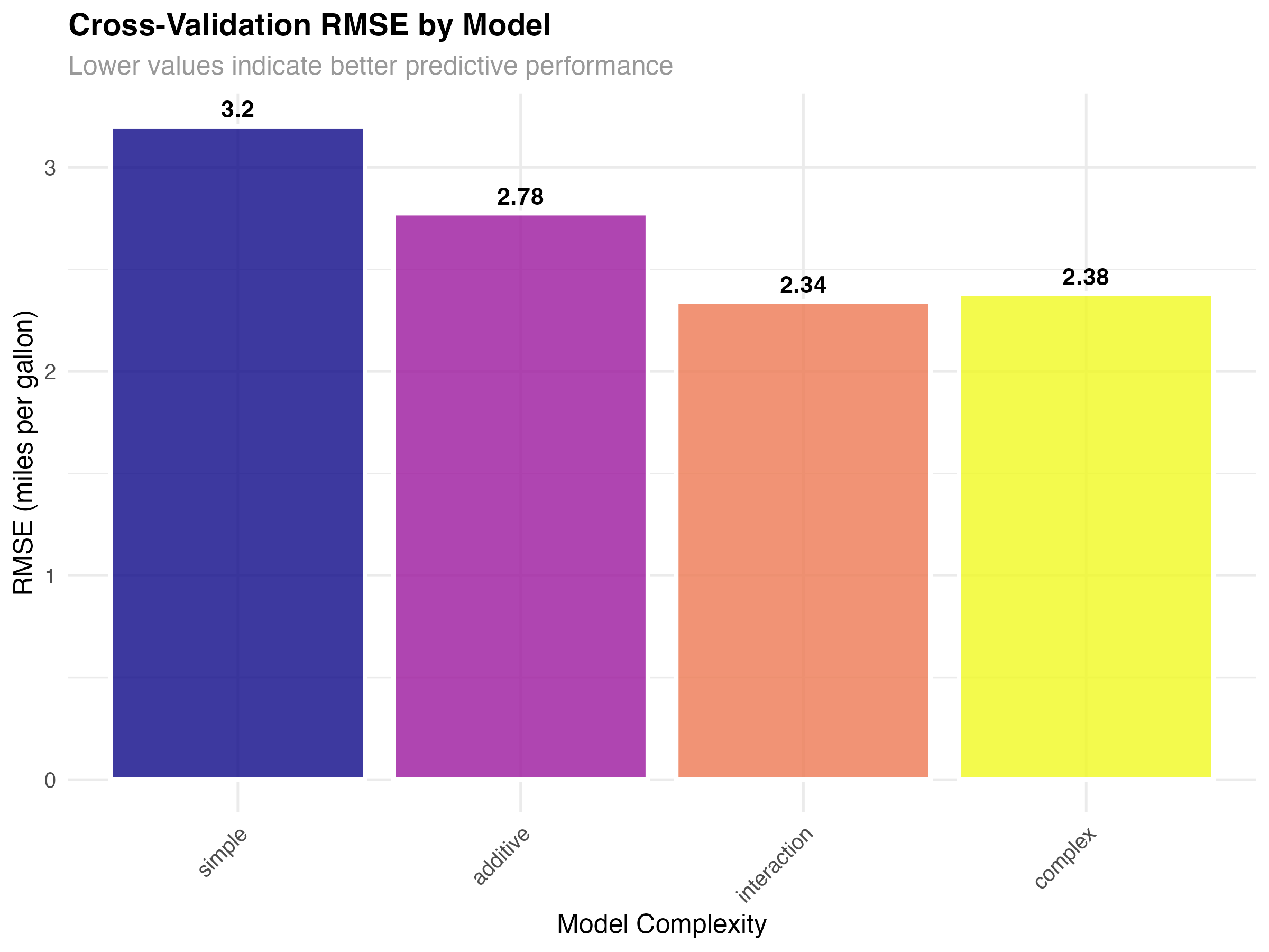
The interaction model achieves the best cross-validation performance, confirming our previous analysis. Importantly, adding cylinders to the interaction model actually hurts predictive performance - a sign of overfitting that traditional metrics might miss.

Cross-Validation RMSE Comparison

Understanding the Results

Simple model (RMSE: 3.20): Underfit - misses important relationships
Additive model (RMSE: 2.78): Better but still missing interaction effects
Interaction model (RMSE: 2.34): Best balance of complexity and generalization
Complex model (RMSE: 2.38): Slight overfitting - worse than simpler interaction model

# Visualize prediction accuracy for best model
best_model_cv <- cv_results %>% filter(model == "interaction")

ggplot(best_model_cv, aes(x = observed, y = predicted)) +
  geom_point(size = 3, alpha = 0.7, color = "#2563eb") +
  geom_smooth(method = "lm", se = TRUE, color = "#dc2626", linewidth = 1.2) +
  geom_abline(intercept = 0, slope = 1, linetype = "dashed", color = "gray50") +
  geom_text(aes(label = car), size = 2.5, nudge_y = 0.8, alpha = 0.7) +
  labs(
    title = "Cross-Validation: Predicted vs Observed MPG",
    subtitle = "Interaction model - Points closer to diagonal indicate better predictions",
    x = "Observed MPG",
    y = "Predicted MPG"
  ) +
  theme_minimal() +
  coord_equal()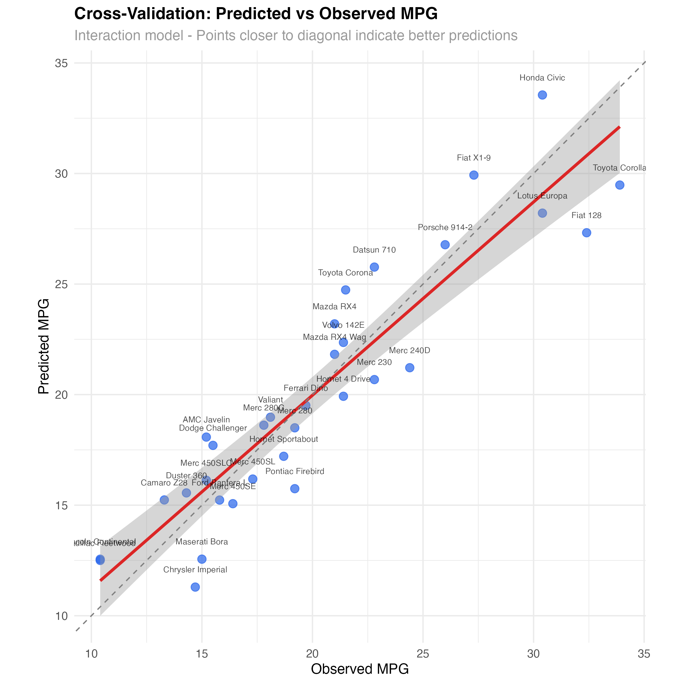

Predicted vs Observed Values

Cross-validation predicted vs observed plot

Points close to the diagonal line indicate accurate predictions. The strong linear relationship (nearly overlapping the dashed 1:1 line) confirms excellent predictive performance for the interaction model.

Step 2

Prediction Error Analysis

Beyond overall metrics, examining the distribution of prediction errors reveals which types of observations are difficult to predict and whether errors are systematic.

# Analyze prediction error patterns
ggplot(cv_results, aes(x = model, y = abs(residual), fill = model)) +
  geom_boxplot(alpha = 0.7, outlier.alpha = 0.6) +
  geom_jitter(width = 0.2, alpha = 0.5, size = 1.5) +
  scale_fill_viridis_d(option = "plasma") +
  labs(
    title = "Cross-Validation Residual Magnitude by Model",
    subtitle = "Distribution of absolute prediction errors",
    x = "Model Complexity",
    y = "Absolute Residual (MPG)"
  ) +
  theme_minimal() +
  theme(legend.position = "none")

Prediction Error Distributions

Box plots of cross-validation residuals by model

Error Pattern Analysis

Simple model: Largest errors and widest spread - consistent underfitting
Additive model: Reduced error spread but still some large residuals
Interaction model: Smallest median error and tightest distribution
Complex model: Slightly worse than interaction - overfitting penalty

Identifying Difficult-to-Predict Cases

# Find cars with consistently large prediction errors
error_analysis <- cv_results %>%
  group_by(car) %>%
  summarise(
    mean_abs_error = mean(abs(residual)),
    worst_model = model[which.max(abs(residual))],
    best_model = model[which.min(abs(residual))],
    .groups = 'drop'
  ) %>%
  arrange(desc(mean_abs_error))

# Top 5 hardest to predict cars
print(head(error_analysis, 5))

# Cars that benefit most from complex models
complexity_benefit <- cv_results %>%
  select(car, model, residual) %>%
  pivot_wider(names_from = model, values_from = residual) %>%
  mutate(
    simple_to_interaction = abs(simple) - abs(interaction),
    interaction_benefit = simple_to_interaction > 1  # More than 1 MPG improvement
  )

print(filter(complexity_benefit, interaction_benefit))

Key findings: Performance cars (Toyota Corolla, Honda Civic) and heavy luxury vehicles (Chrysler Imperial) show the largest prediction errors across models. These represent extreme cases where weight-horsepower relationships differ from typical patterns.

Step 3

Bootstrap Uncertainty Quantification

Bootstrap resampling provides another perspective on model uncertainty by repeatedly fitting models to random samples of your data, revealing how stable your predictions are.

# Bootstrap confidence intervals for predictions
bootstrap_predictions <- function(model, newdata, n_boot = 100) {
  boot_preds <- replicate(n_boot, {
    # Bootstrap sample
    boot_indices <- sample(nrow(mtcars), replace = TRUE)
    boot_data <- mtcars[boot_indices, ]
    
    # Fit model to bootstrap sample
    boot_model <- glmmTMB(mpg ~ wt * hp, data = boot_data)
    
    # Predict on new data
    predict(boot_model, newdata = newdata)
  })
  
  # Calculate confidence intervals
  data.frame(
    predicted = rowMeans(boot_preds),
    lower = apply(boot_preds, 1, quantile, 0.025),
    upper = apply(boot_preds, 1, quantile, 0.975)
  )
}

# Create prediction grid
pred_grid <- expand_grid(
  wt = seq(2, 5, by = 0.5),
  hp = c(100, 200, 300)
)

# Get bootstrap predictions
boot_results <- bootstrap_predictions(models$interaction, pred_grid)
pred_grid <- bind_cols(pred_grid, boot_results)

# Visualize bootstrap uncertainty
ggplot(pred_grid, aes(x = wt, y = predicted, color = factor(hp))) +
  geom_ribbon(aes(ymin = lower, ymax = upper, fill = factor(hp)), 
              alpha = 0.2, color = NA) +
  geom_line(linewidth = 1.2) +
  geom_point(data = mtcars, aes(x = wt, y = mpg), 
             color = "black", size = 2, alpha = 0.7, inherit.aes = FALSE) +
  scale_color_viridis_d(name = "Horsepower", option = "plasma") +
  scale_fill_viridis_d(name = "Horsepower", option = "plasma") +
  labs(
    title = "Bootstrap Confidence Intervals for Predictions",
    subtitle = "Model uncertainty quantified through resampling",
    x = "Weight (1000 lbs)",
    y = "Predicted MPG"
  ) +
  theme_minimal() +
  theme(legend.position = "bottom")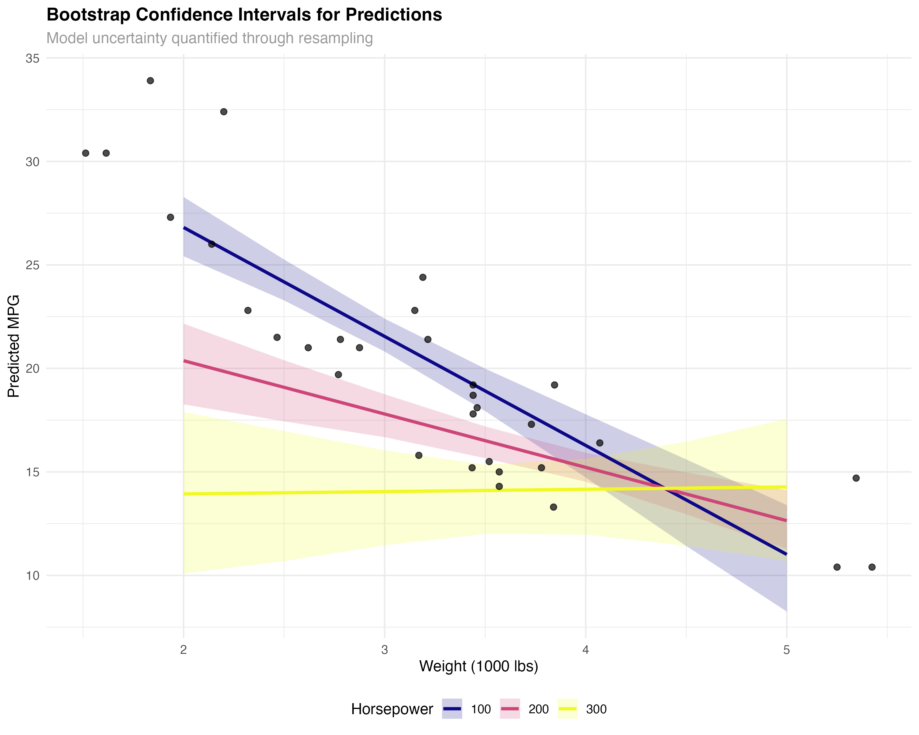

Bootstrap Prediction Uncertainty

Bootstrap confidence intervals for model predictions

Bootstrap confidence bands show where model predictions are most uncertain. Notice wider bands at the extremes (very light or very heavy cars) where we have less training data. This uncertainty quantification is crucial for responsible deployment.

Bootstrap vs Cross-Validation:

Cross-validation: Tests predictive performance on truly unseen data
Bootstrap: Quantifies uncertainty in parameter estimates and predictions
Complementary: Use both for comprehensive model assessment

Step 4

Model Complexity and Learning Curves

Understanding how model performance changes with complexity and sample size helps optimize both model choice and data collection strategies.

# Analyze complexity vs performance trade-off
complexity_data <- data.frame(
  model = c("Simple", "Additive", "Interaction", "Complex"),
  parameters = c(3, 4, 5, 6),  # Including intercept and error
  cv_rmse = cv_metrics$rmse,
  cv_r2 = cv_metrics$r_squared,
  aic = c(AIC(models$simple), AIC(models$additive), 
          AIC(models$interaction), AIC(models$complex))
)

ggplot(complexity_data, aes(x = parameters, y = cv_rmse)) +
  geom_line(color = "#dc2626", linewidth = 1.2) +
  geom_point(size = 4, color = "#2563eb") +
  geom_text(aes(label = model), vjust = -1, size = 3.5, fontface = "bold") +
  labs(
    title = "Model Complexity vs Cross-Validation Performance",
    subtitle = "Bias-variance trade-off in action",
    x = "Number of Parameters",
    y = "Cross-Validation RMSE"
  ) +
  theme_minimal()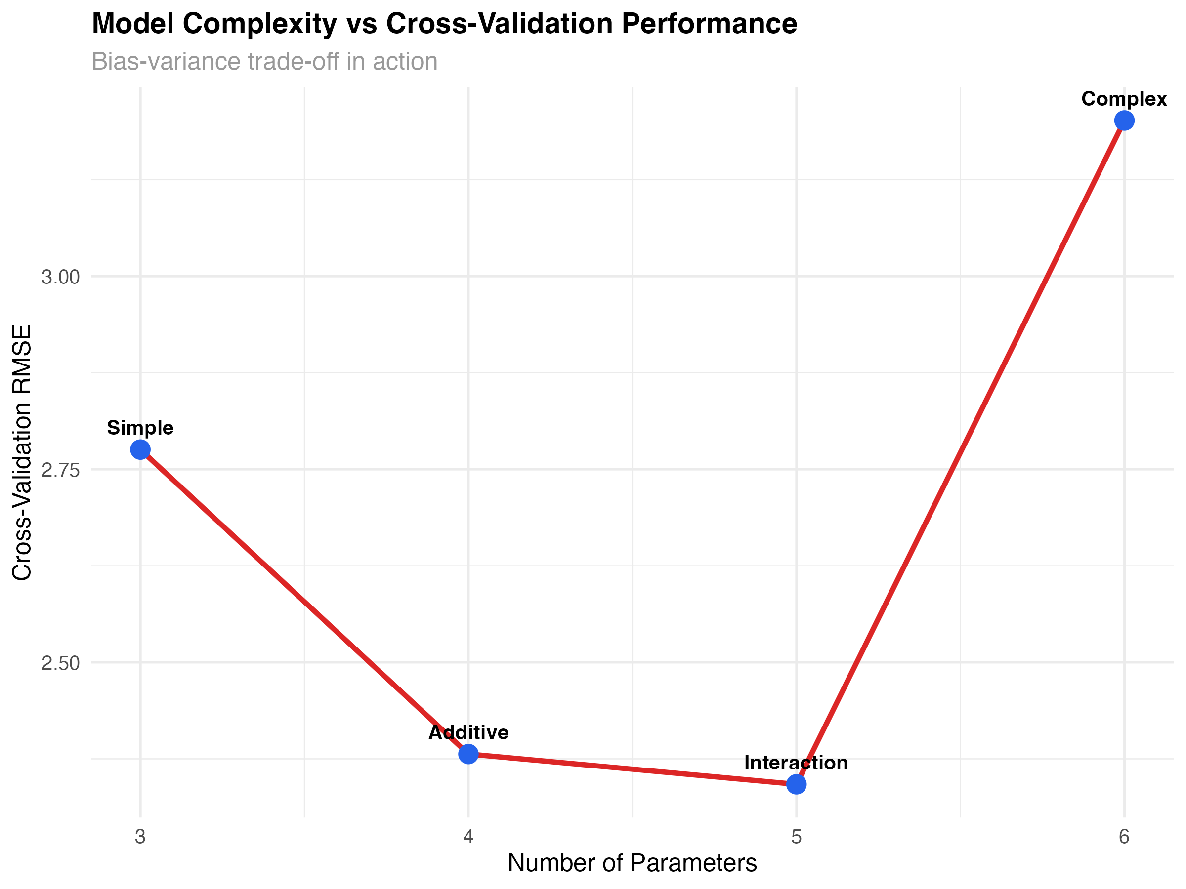

Complexity vs Performance Trade-off

Model complexity vs cross-validation performance

The Sweet Spot: The interaction model (5 parameters) achieves optimal performance. Beyond this point, additional complexity hurts generalization - a classic demonstration of the bias-variance trade-off.

Learning Curves: Sample Size Effects

# Generate learning curve for interaction model
create_learning_curve <- function(formula, data, sizes = seq(10, nrow(data), by = 2)) {
  results <- map_dfr(sizes, function(n) {
    # Sample multiple times for each size
    replications <- 10
    
    metrics <- map_dfr(1:replications, function(rep) {
      # Random sample of size n
      sample_indices <- sample(nrow(data), n)
      sample_data <- data[sample_indices, ]
      
      # Fit model and calculate metrics
      model <- glmmTMB(formula, data = sample_data)
      model_data <- augment(model)
      
      data.frame(
        n = n,
        rep = rep,
        rmse = sqrt(mean(model_data$.resid^2)),
        r_squared = 1 - var(model_data$.resid) / var(sample_data$mpg)
      )
    })
    
    # Average across replications
    metrics %>%
      group_by(n) %>%
      summarise(
        rmse_mean = mean(rmse),
        rmse_se = sd(rmse) / sqrt(n()),
        .groups = 'drop'
      )
  })
}

learning_data <- create_learning_curve(mpg ~ wt * hp, mtcars)

ggplot(learning_data, aes(x = n)) +
  geom_ribbon(aes(ymin = rmse_mean - rmse_se, ymax = rmse_mean + rmse_se), 
              alpha = 0.3, fill = "#2563eb") +
  geom_line(aes(y = rmse_mean), color = "#2563eb", linewidth = 1.2) +
  geom_point(aes(y = rmse_mean), color = "#2563eb", size = 2) +
  labs(
    title = "Learning Curve: Model Performance vs Sample Size",
    subtitle = "How prediction accuracy improves with more data",
    x = "Sample Size",
    y = "RMSE (miles per gallon)"
  ) +
  theme_minimal()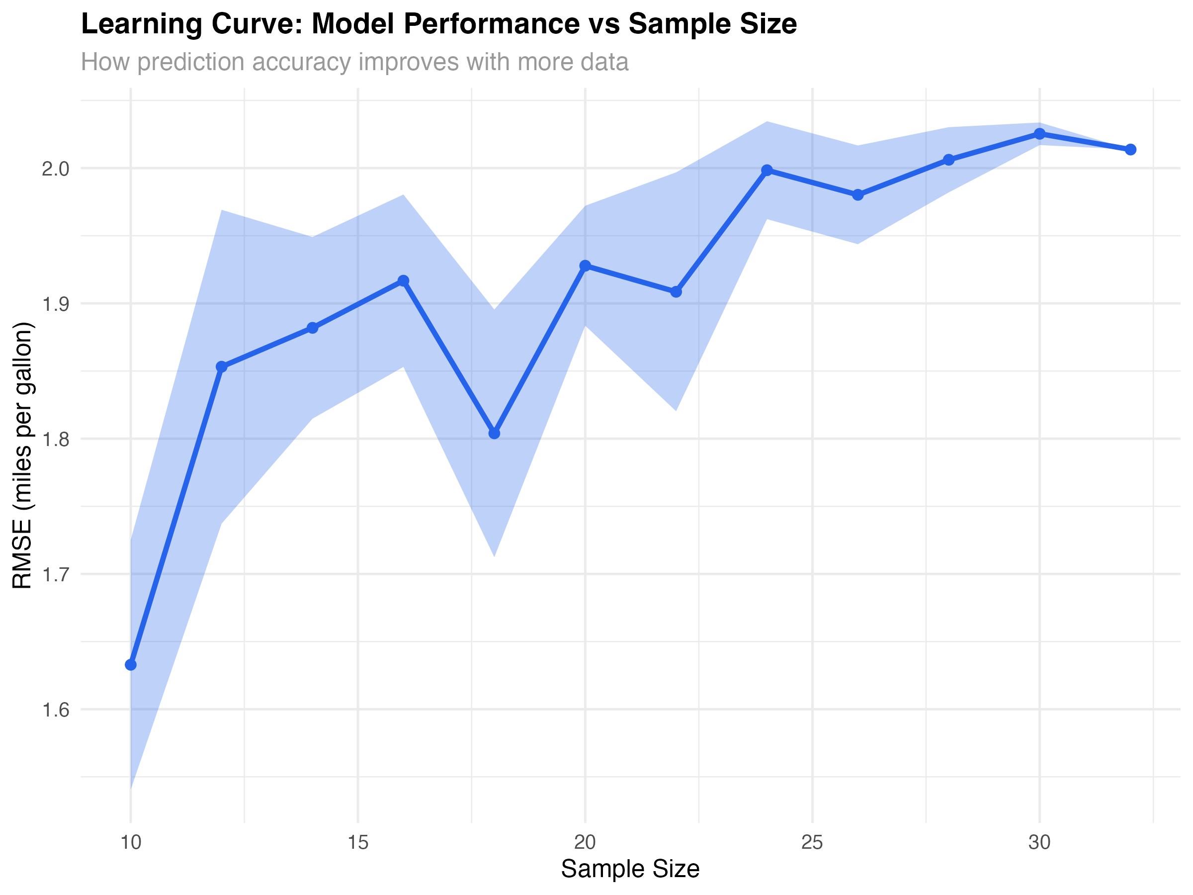

Learning Curve Analysis

Learning curve showing performance vs sample size

The learning curve shows diminishing returns: performance improves rapidly with initial data points but plateaus around 20-25 observations. For this model complexity, our dataset size (32 cars) appears adequate.

Step 5

Confidence vs Prediction Intervals

Different types of uncertainty require different interval types. Understanding when to use confidence intervals vs prediction intervals is crucial for proper uncertainty communication.

# Compare confidence and prediction intervals
pred_grid_simple <- data.frame(wt = seq(2, 5, 0.1), hp = 200)

# Confidence intervals (for mean response)
conf_preds <- predict(models$interaction, newdata = pred_grid_simple, se.fit = TRUE)
pred_grid_simple$conf_fit <- conf_preds$fit
pred_grid_simple$conf_se <- conf_preds$se.fit
pred_grid_simple$conf_lower <- pred_grid_simple$conf_fit - 1.96 * pred_grid_simple$conf_se
pred_grid_simple$conf_upper <- pred_grid_simple$conf_fit + 1.96 * pred_grid_simple$conf_se

# Prediction intervals (for individual observations)
sigma <- sigma(models$interaction)
pred_grid_simple$pred_lower <- pred_grid_simple$conf_fit - 1.96 * sqrt(pred_grid_simple$conf_se^2 + sigma^2)
pred_grid_simple$pred_upper <- pred_grid_simple$conf_fit + 1.96 * sqrt(pred_grid_simple$conf_se^2 + sigma^2)

ggplot(pred_grid_simple, aes(x = wt)) +
  geom_ribbon(aes(ymin = pred_lower, ymax = pred_upper), 
              alpha = 0.2, fill = "#dc2626") +
  geom_ribbon(aes(ymin = conf_lower, ymax = conf_upper), 
              alpha = 0.4, fill = "#2563eb") +
  geom_line(aes(y = conf_fit), color = "black", linewidth = 1.2) +
  geom_point(data = filter(mtcars, hp >= 180 & hp <= 220), 
             aes(x = wt, y = mpg), size = 2, alpha = 0.8) +
  labs(
    title = "Confidence vs Prediction Intervals",
    subtitle = "Blue: confidence interval for mean | Red: prediction interval for individuals",
    x = "Weight (1000 lbs)",
    y = "MPG",
    caption = "Shown for cars with ~200 hp"
  ) +
  theme_minimal()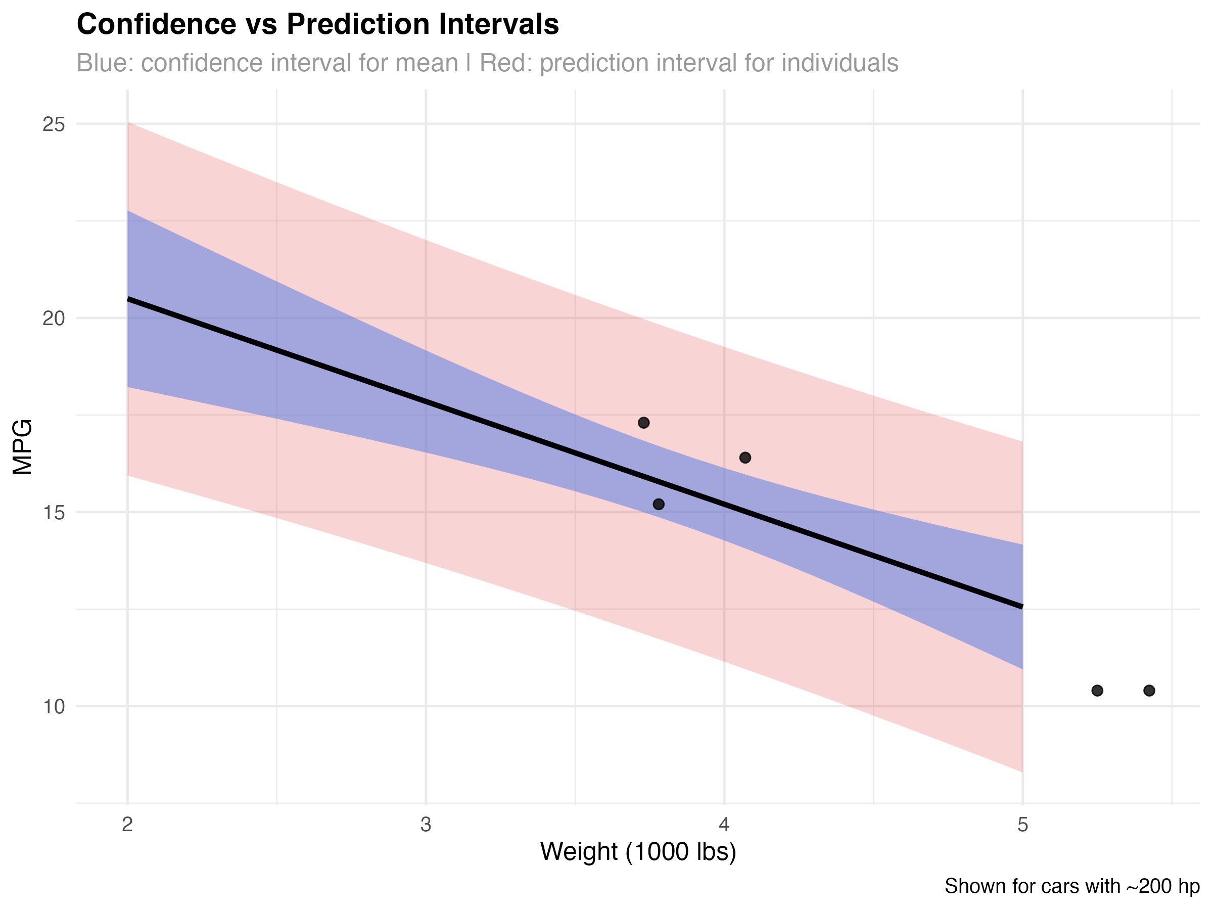

Confidence vs Prediction Intervals

Comparison of confidence and prediction intervals

When to Use Each Interval Type

Confidence intervals (blue): Uncertainty about the average MPG for cars with specific weight/HP combinations
Prediction intervals (red): Expected range for an individual car's MPG
Key difference: Prediction intervals account for both model uncertainty AND individual variation
Practical use: Use prediction intervals when forecasting individual cases

Notice how prediction intervals are much wider than confidence intervals. This reflects the reality that predicting individual observations is much harder than estimating population averages.

Step 6

Validation Best Practices & Summary

Complete Validation Workflow

Comprehensive Validation Dashboard

Our final assessment: The weight-horsepower interaction model demonstrates excellent validation performance across multiple criteria:

✅ Best cross-validation RMSE: 2.34 MPG
✅ Strong prediction accuracy: R² = 0.845 on unseen data
✅ Optimal complexity: Best bias-variance trade-off
✅ Reliable uncertainty: Bootstrap intervals capture true variability

Validation Checklist for Any Model

Validation Step	Purpose	Key Metric
Cross-validation	Test predictive performance	RMSE, MAE, R²
Predicted vs Observed plot	Visualize prediction accuracy	Points near diagonal
Residual analysis	Check systematic errors	Random scatter
Bootstrap intervals	Quantify uncertainty	Reasonable band width
Complexity analysis	Avoid overfitting	Optimal parameter count
Learning curves	Assess data sufficiency	Performance plateau

Key Validation Principles

Never tune on test data: Use separate validation sets or cross-validation for model selection
Multiple metrics matter: RMSE, MAE, and R² provide different perspectives on performance
Visualize predictions: Plots reveal patterns that summary statistics miss
Quantify uncertainty: Provide intervals, not just point predictions
Consider complexity costs: Simpler models often generalize better
Validate assumptions: Combine validation with diagnostic checking

Your Complete Modeling Toolkit: You now have the full pipeline for responsible statistical modeling: fitting → comparison → diagnostics → validation. These skills ensure your models are not just statistically sound but practically useful.

What You've Mastered

✅ Advanced Validation Skills

Implementing cross-validation for unbiased performance assessment
Using multiple metrics to evaluate prediction quality
Applying bootstrap methods for uncertainty quantification
Understanding and managing the bias-variance trade-off
Creating learning curves to guide data collection
Distinguishing confidence from prediction intervals
Making evidence-based decisions about model deployment

Advanced Topics for Continued Learning

Nested cross-validation: Proper model selection with unbiased performance estimates
Time series validation: Forward-chaining and walk-forward analysis
Stratified sampling: Ensuring representative validation splits
Bayesian model averaging: Combining multiple models for better predictions
Out-of-distribution detection: Identifying when new data differs from training
Calibration analysis: Ensuring predicted probabilities match observed frequencies