Welcome to the rstatix Ecosystem
Your gateway to streamlined statistical analysis in R
If you've ever found yourself drowning in a sea of different R packages for statistical testing—each with its own syntax, output format, and quirks—then rstatix is about to become your new best friend. Created by Alboukadel Kassambara, the mastermind behind the beloved ggpubr package, rstatix was born from a simple but powerful idea: statistical analysis should be as intuitive and consistent as the tidyverse workflow you already love.
🤔 Why Does rstatix Matter?
Picture this scenario: You're analyzing a multi-center clinical trial with 800 patients across 4 treatment groups. You need to:
- Run descriptive statistics by treatment and center
- Perform ANOVA with post-hoc comparisons
- Check normality assumptions for each group
- Calculate effect sizes with confidence intervals
- Apply different multiple comparison corrections
- Create publication-ready plots with statistical annotations
Without rstatix, you'd be juggling functions from base R, stats, broom, effsize, multcomp, and half a dozen other packages—each with different output formats, different parameter names, and different ways of handling grouped data. With rstatix, it's all unified under one consistent, tidy framework.
🎯 The rstatix Philosophy
🧹 Tidy First
Every function returns a clean data frame that plays nicely with dplyr, ggplot2, and the rest of the tidyverse ecosystem.
👥 Group-Aware
Built-in support for grouped analysis using group_by()—no more manual data splitting or loop writing.
📊 Visualization-Ready
Seamless integration with ggpubr for automatic statistical annotations on your plots.
🔧 Comprehensive
From basic t-tests to complex ANOVA designs, from normality testing to effect sizes—all in one unified package.
💡 Real-World Impact
Before rstatix: "Let me check if this is the right function... wait, why is the output a list? How do I extract the p-values? Which package has the effect size function again?"
With rstatix: "Let me just pipe my grouped data through the statistical test function and directly into my plotting function. Done."
This isn't just about convenience—it's about reducing errors, improving reproducibility, and letting you focus on the science instead of wrestling with syntax.
🧪 What You'll Learn Today
We'll walk through a comprehensive analysis of a simulated multi-center hypertension trial, demonstrating how rstatix transforms complex statistical workflows into elegant, readable code. You'll see how to:
get_summary_stats(), anova_test(), pairwise_t_test(), and friends
Multi-center, multi-arm trials with nested grouping structures
Bonferroni, FDR, Holm—when to use what and why it matters
Statistical annotations that reviewers will love
Ready to transform your statistical analysis workflow? Let's dive into the world of tidy statistical testing with rstatix. 🚀
🎯 Learning Objectives: Mastering rstatix
📊 Case Study: Multi-Center Hypertension Trial Analysis with rstatix
A comprehensive demonstration of rstatix capabilities using a simulated 8-center, 4-arm hypertension trial with 800 patients and complex group-wise statistical testing requirements
rstatix Function Ecosystem
Comprehensive statistical testing with tidy output
🔧 Core rstatix Functions
library(tidyverse)
library(rstatix)
library(ggpubr)
library(glmmTMB)
library(broom)

# Load simulated multi-center hypertension trial data
# 800 patients across 8 centers, 4 treatment arms
# Primary endpoint: Systolic BP at Month 6

# Key grouping variables for rstatix analysis:
# - treatment: Placebo, ACE_Inhibitor, ARB, Combination
# - center_name: 8 clinical centers (A through H)
# - age_group: Young (<50), Middle (50-65), Older (>65)
# - risk_category: Standard_Risk, Moderate_Risk, High_Risk

# Primary analysis dataset (Month 6 - primary endpoint)
primary_analysis_data <- longitudinal_data %>%
  filter(timepoint == "Month_6") %>%
  mutate(
    age_group = case_when(
      age < 50 ~ "Young",
      age < 65 ~ "Middle",
      TRUE ~ "Older"
    ),
    risk_category = case_when(
      diabetes != "No" | baseline_sbp >= 180 ~ "High_Risk",
      baseline_sbp >= 160 ~ "Moderate_Risk",
      TRUE ~ "Standard_Risk"
    )
)- get_summary_stats() with type options
- Group-wise summaries with group_by()
- Multiple variables simultaneously
- Custom statistic selection
- Tidy output format
- anova_test() for group comparisons
- Automatic effect size calculation
- Two-way ANOVA with interactions
- ANCOVA with covariates
- Repeated measures support
- pairwise_t_test() with corrections
- tukey_hsd() for balanced designs
- Bonferroni, FDR, Holm methods
- Group-wise corrections
- adjust_pvalue() for custom corrections
- kruskal_test() for non-normal data
- wilcox_test() for pairwise comparisons
- dunn_test() for post-hoc analysis
- Rank-based alternatives
- Ordinal data support
Statistical Testing with Visual Annotations
ggpubr integration for publication-ready plots
# ANOVA with post-hoc comparisons
anova_sbp <- primary_analysis_data %>%
  anova_test(sbp ~ treatment)

# Pairwise comparisons with FDR correction
posthoc_sbp_fdr <- primary_analysis_data %>%
  pairwise_t_test(sbp ~ treatment, p.adjust.method = "fdr")

# Create box plot with statistical annotations
ggboxplot(primary_analysis_data, x = "treatment", y = "sbp",
          color = "treatment", palette = "viridis",
          add = "jitter", add.params = list(alpha = 0.3)) +
  stat_compare_means(method = "anova", label.y = 200, size = 4) +
  stat_compare_means(comparisons = list(
    c("Placebo", "ACE_Inhibitor"),
    c("Placebo", "ARB"),
    c("Placebo", "Combination"),
    c("ACE_Inhibitor", "Combination"),
    c("ARB", "Combination")
  ), method = "t.test",
  p.adjust.method = "fdr",
  label = "p.signif",
  step.increase = 0.08)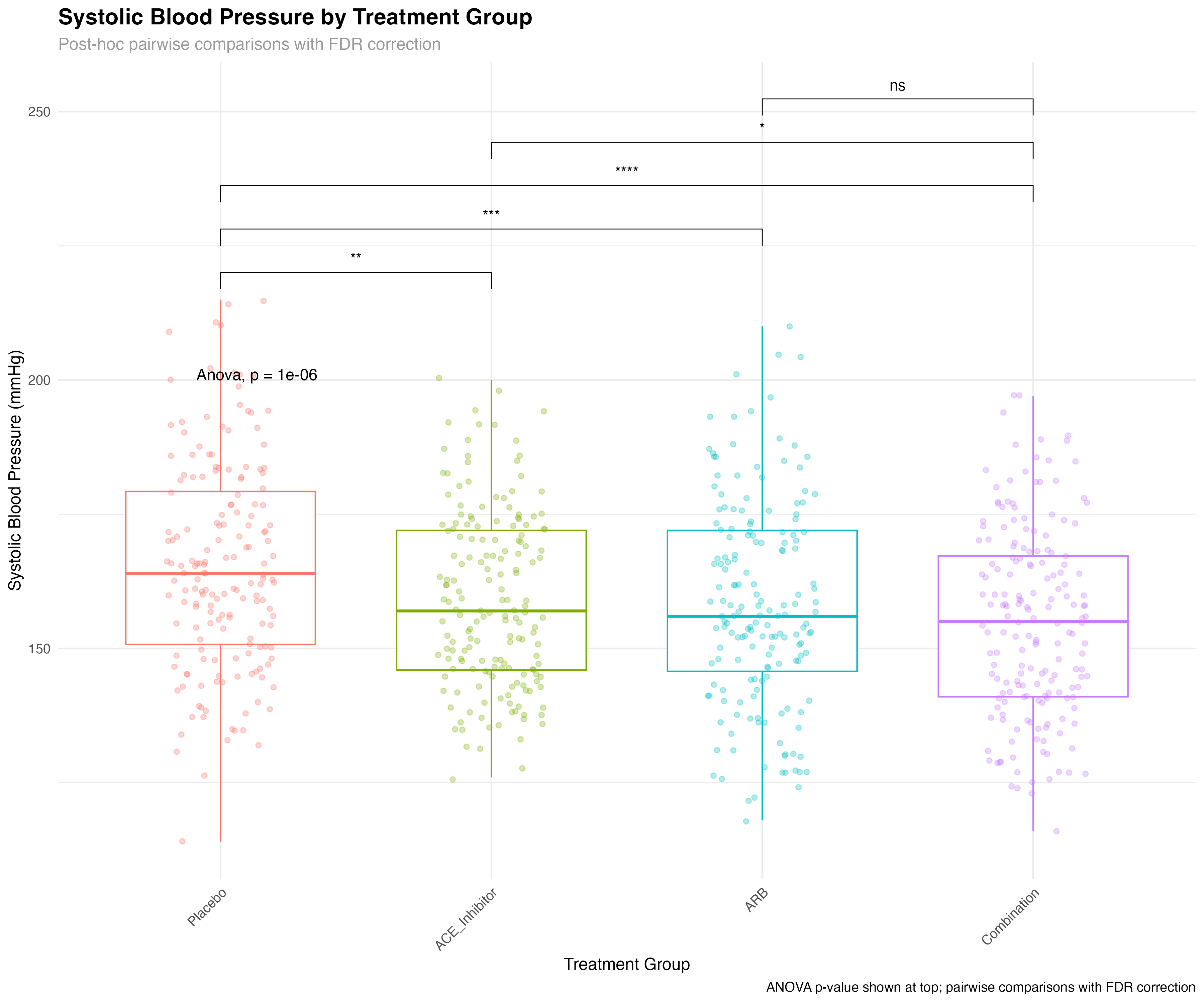
⚡ rstatix + ggpubr Advantage
The integration between rstatix and ggpubr provides unmatched efficiency for statistical visualization. Instead of manually calculating p-values and adding annotations, stat_compare_means() automatically performs the appropriate tests, applies corrections, and displays results directly on plots. This reduces errors, saves time, and ensures consistency across analyses.
Multiple Comparison Correction Methods
Comprehensive approach to p-value adjustment
# Compare different multiple comparison correction methods
posthoc_sbp_bonferroni <- primary_analysis_data %>%
  pairwise_t_test(sbp ~ treatment, p.adjust.method = "bonferroni")

posthoc_sbp_fdr <- primary_analysis_data %>%
  pairwise_t_test(sbp ~ treatment, p.adjust.method = "fdr")

posthoc_sbp_holm <- primary_analysis_data %>%
  pairwise_t_test(sbp ~ treatment, p.adjust.method = "holm")

# Combine results for comparison
comparison_methods <- bind_rows(
  posthoc_sbp_bonferroni %>% mutate(method = "Bonferroni"),
  posthoc_sbp_fdr %>% mutate(method = "FDR"),
  posthoc_sbp_holm %>% mutate(method = "Holm")
) %>%
  mutate(
    comparison = paste(group1, "vs", group2),
    significant = case_when(
      p.adj < 0.001 ~ "***",
      p.adj < 0.01 ~ "**",
      p.adj < 0.05 ~ "*",
      TRUE ~ "ns"
    ),
    log_p_adj = -log10(p.adj)
  )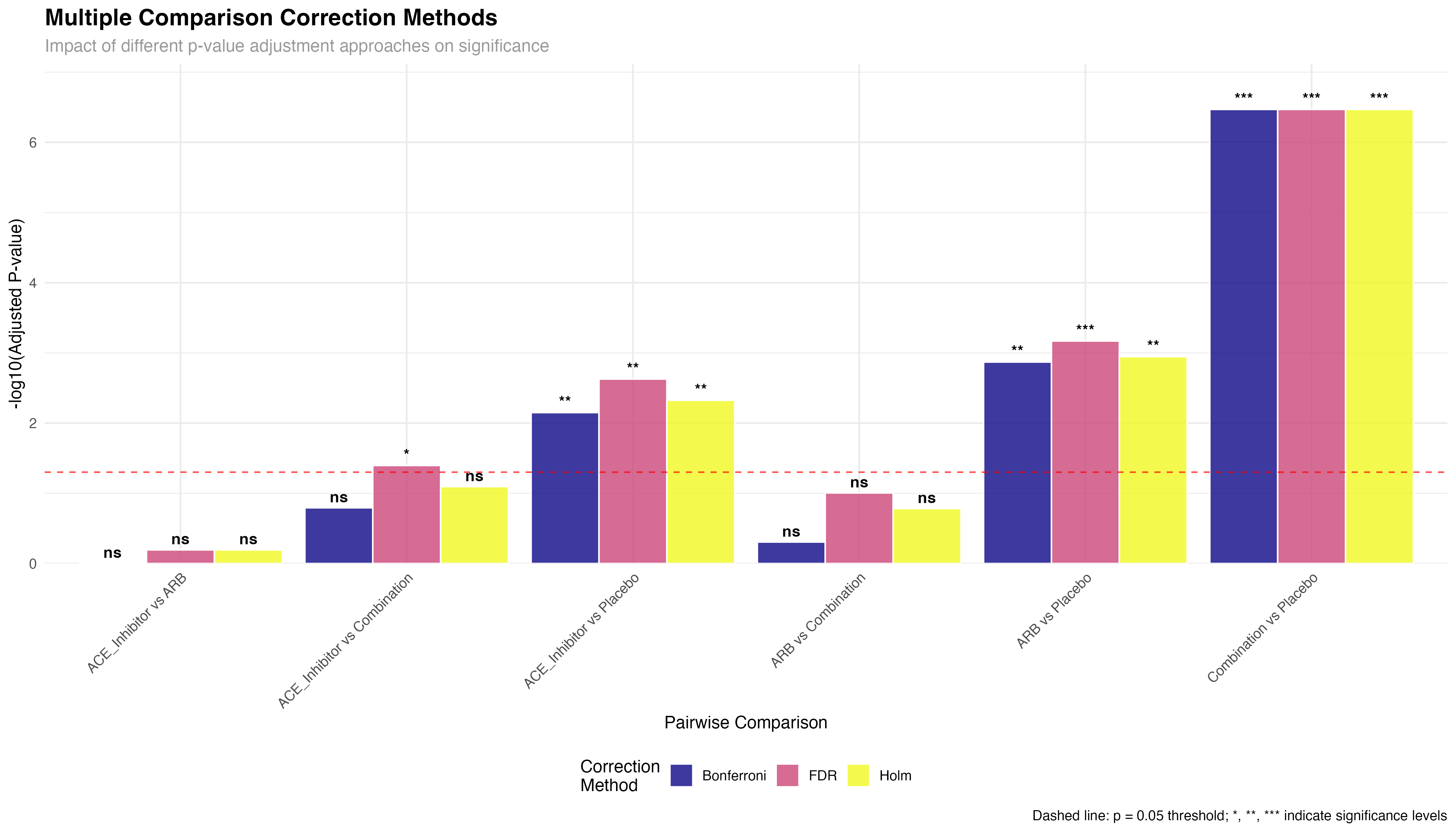
| Correction Method | Type | Conservatism | Use Case | rstatix Function |
|---|---|---|---|---|
| Bonferroni | Family-wise Error Rate | Very Conservative | Strong Type I error control | p.adjust.method = "bonferroni" |
| Holm | Family-wise Error Rate | Conservative | Uniformly more powerful than Bonferroni | p.adjust.method = "holm" |
| FDR (Benjamini-Hochberg) | False Discovery Rate | Moderate | Exploratory analysis, many comparisons | p.adjust.method = "fdr" |
| None | No correction | Not conservative | Single planned comparison only | p.adjust.method = "none" |
📐 Choosing Correction Methods
Method selection depends on research goals: Bonferroni/Holm for confirmatory analysis requiring strong Type I error control; FDR for exploratory analysis or large-scale screening where some false positives are acceptable; No correction only for single, pre-planned comparisons. rstatix makes it easy to compare methods and document the rationale for your choice.
Group-wise Multiple Comparisons
Advanced group_by() workflows for complex designs
# Key rstatix feature: group-wise multiple comparisons
# Multiple comparisons within each center
posthoc_by_center <- primary_analysis_data %>%
  group_by(center_name) %>%
  pairwise_t_test(sbp ~ treatment, p.adjust.method = "fdr") %>%
  adjust_pvalue(method = "fdr")  # Additional adjustment across centers

# Multiple comparisons within each age group
posthoc_by_age <- primary_analysis_data %>%
  group_by(age_group) %>%
  pairwise_t_test(sbp ~ treatment, p.adjust.method = "bonferroni")

# Multiple comparisons within each risk category
posthoc_by_risk <- primary_analysis_data %>%
  group_by(risk_category) %>%
  pairwise_t_test(sbp ~ treatment, p.adjust.method = "holm")

# Example: Center-specific treatment effects
cat("Center A treatment comparisons:\n")
posthoc_by_center %>%
  filter(center_name == "Center A", p.adj < 0.05) %>%
  select(group1, group2, p.adj, p.adj.signif) %>%
  print()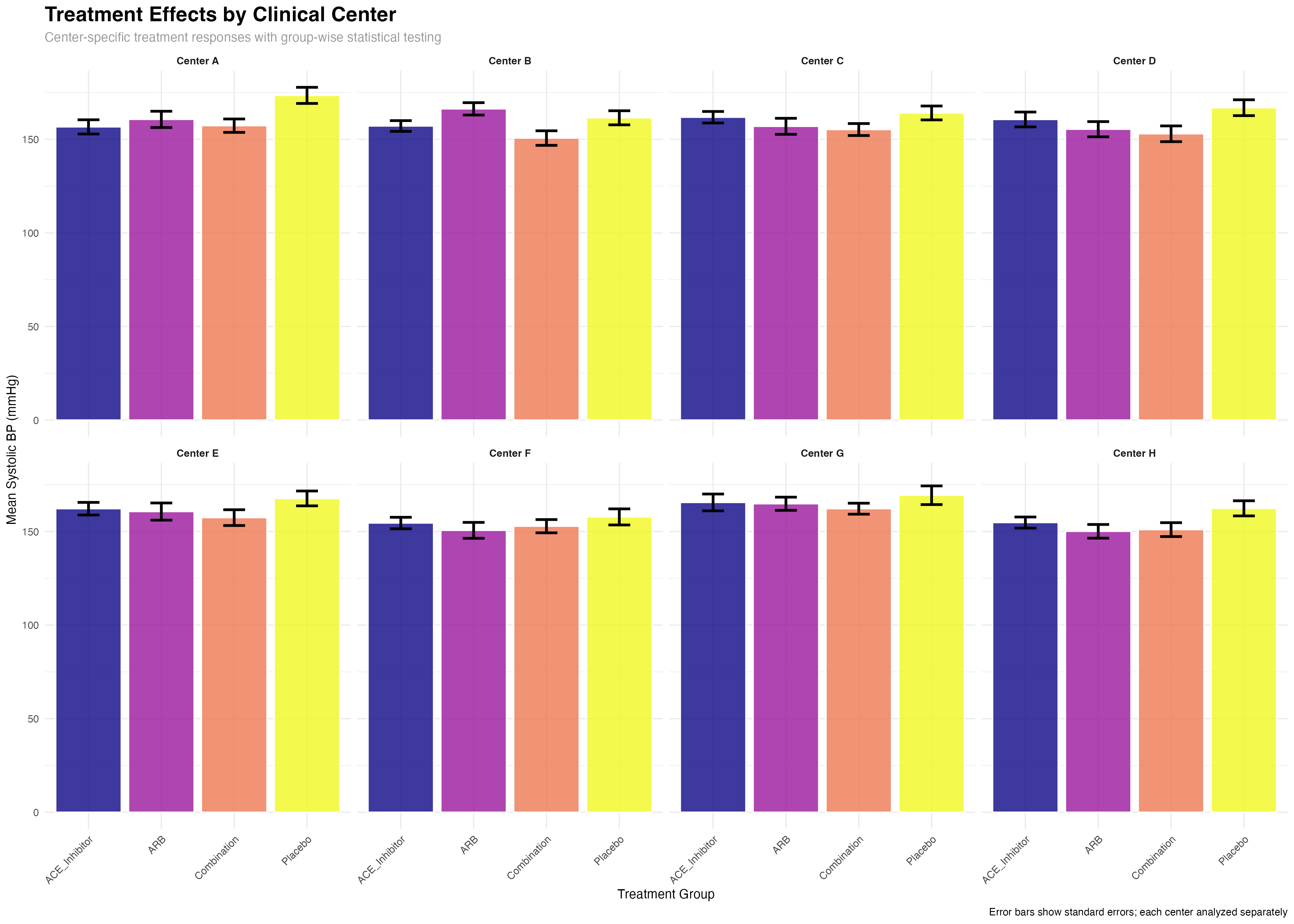
🔄 Group-wise Workflow Benefits
rstatix's group_by() integration enables sophisticated multi-level analyses: (1) Automatic subgroup analysis without manual data splitting; (2) Consistent statistical methods across all groups; (3) Built-in multiple comparison corrections within and across groups; (4) Tidy output format that preserves grouping structure for further analysis and visualization.
Effect Sizes and Practical Significance
Beyond p-values: quantifying clinical importance
# Cohen's d for treatment comparisons
cohens_d_sbp <- primary_analysis_data %>%
  cohens_d(sbp ~ treatment, ref.group = "Placebo")

cohens_d_dbp <- primary_analysis_data %>%
  cohens_d(dbp ~ treatment, ref.group = "Placebo")

# Effect size interpretation
effect_sizes_plot <- cohens_d_sbp %>%
  mutate(
    treatment = factor(group2, levels = treatment_arms[-1]),
    magnitude = case_when(
      abs(effsize) < 0.2 ~ "Negligible",
      abs(effsize) < 0.5 ~ "Small",
      abs(effsize) < 0.8 ~ "Medium",
      TRUE ~ "Large"
    ),
    clinical_significance = case_when(
      abs(effsize) >= 0.5 ~ "Clinically Meaningful",
      abs(effsize) >= 0.2 ~ "Potentially Meaningful",
      TRUE ~ "Minimal Clinical Impact"
    )
  )

# Display results
print(effect_sizes_plot)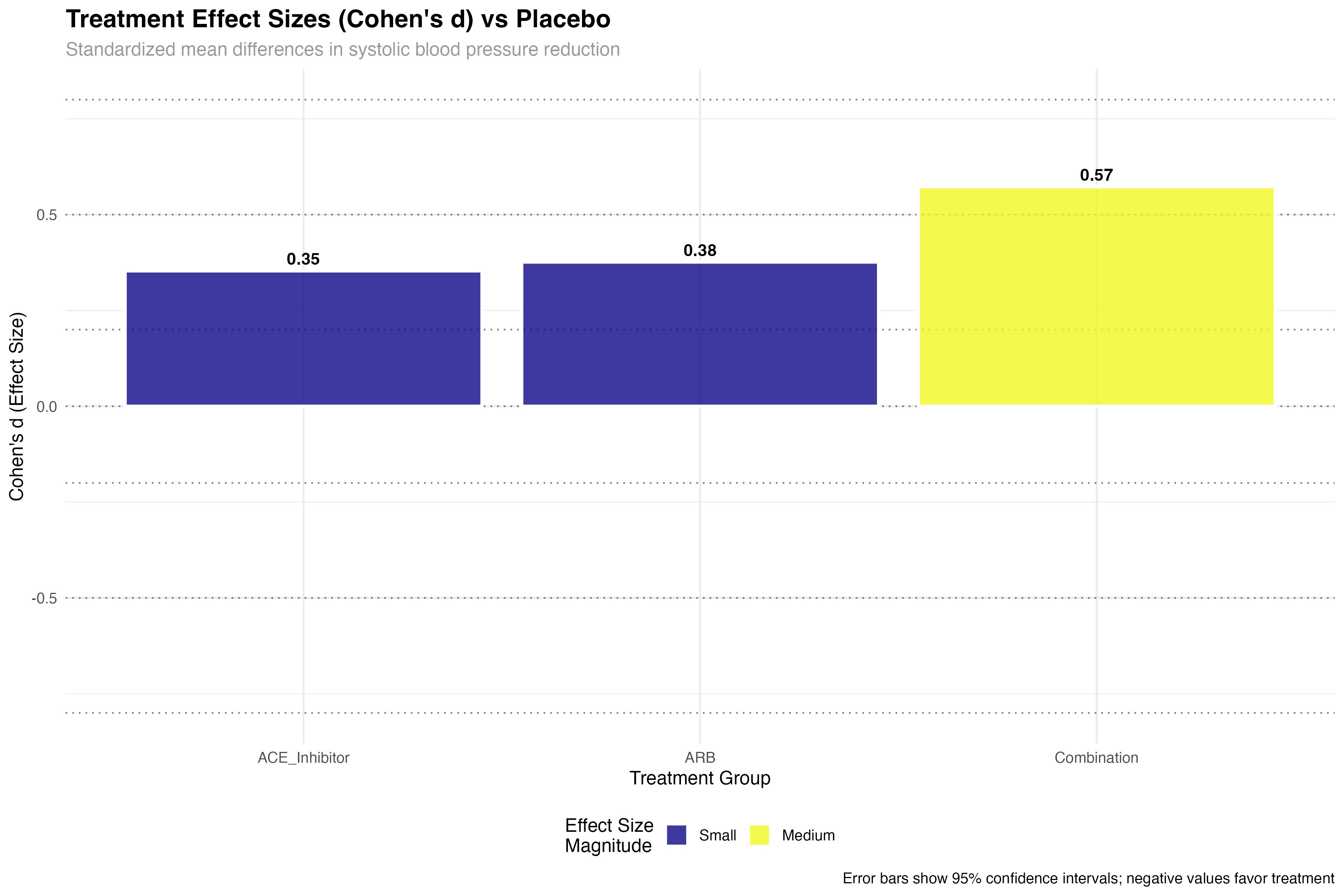
🎯 Clinical Effect Size Interpretation
Effect sizes provide crucial clinical context: Small effects (d = 0.2-0.5) may be meaningful for common conditions or large populations; Medium effects (d = 0.5-0.8) represent clinically important differences; Large effects (d > 0.8) indicate substantial clinical benefits. In hypertension trials, even small effect sizes can translate to significant cardiovascular risk reduction at the population level.
Normality Assessment and Test Selection
Choosing appropriate statistical methods
# Shapiro-Wilk test by groups
normality_tests <- primary_analysis_data %>%
group_by(treatment) %>%
shapiro_test(sbp, dbp, quality_of_life)
# Display normality test results
print(normality_tests)
# Alternative: Anderson-Darling or Kolmogorov-Smirnov
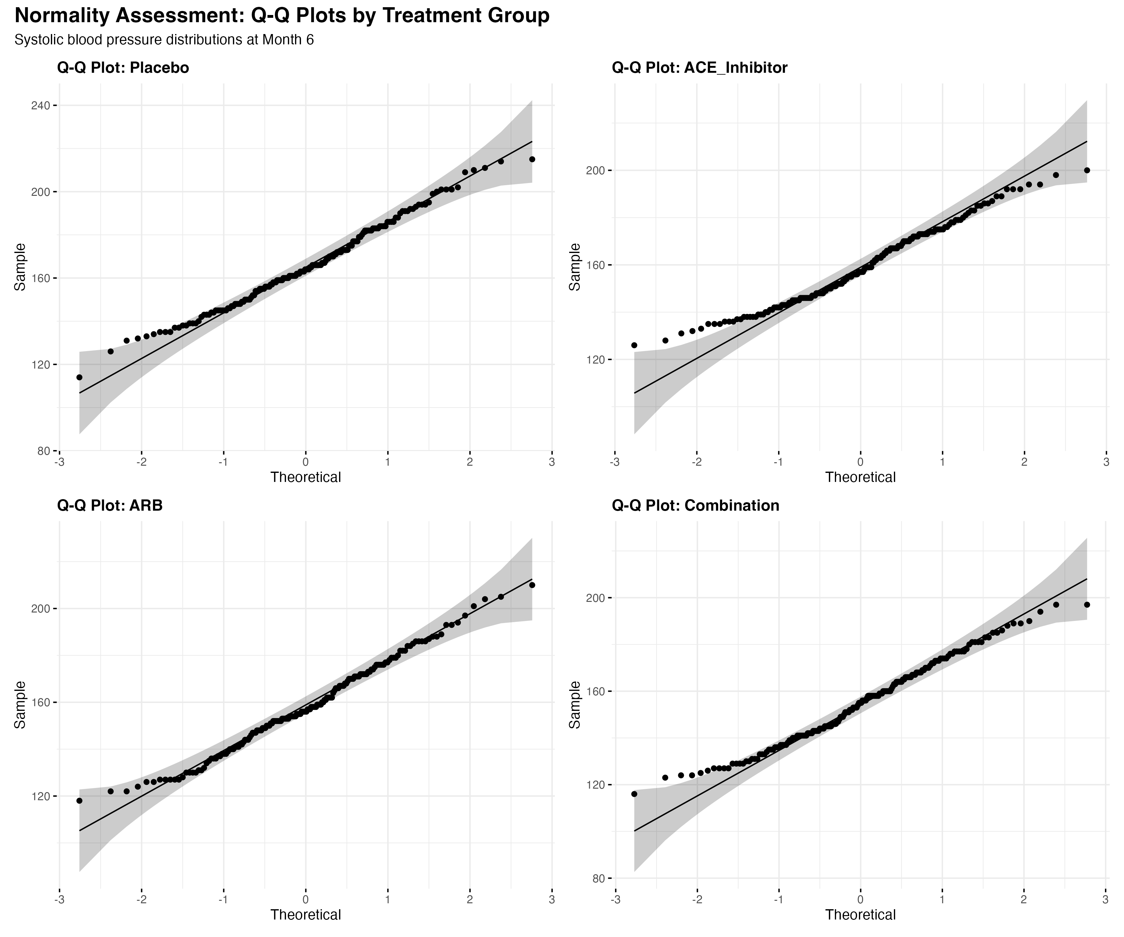
# Q-Q plots for visual assessment
map(treatment_arms, function(trt) {
data_subset <- primary_analysis_data %>% filter(treatment == trt)
ggqqplot(data_subset, x = "sbp",
title = paste("Q-Q Plot:", trt),
ggtheme = theme_minimal())
})
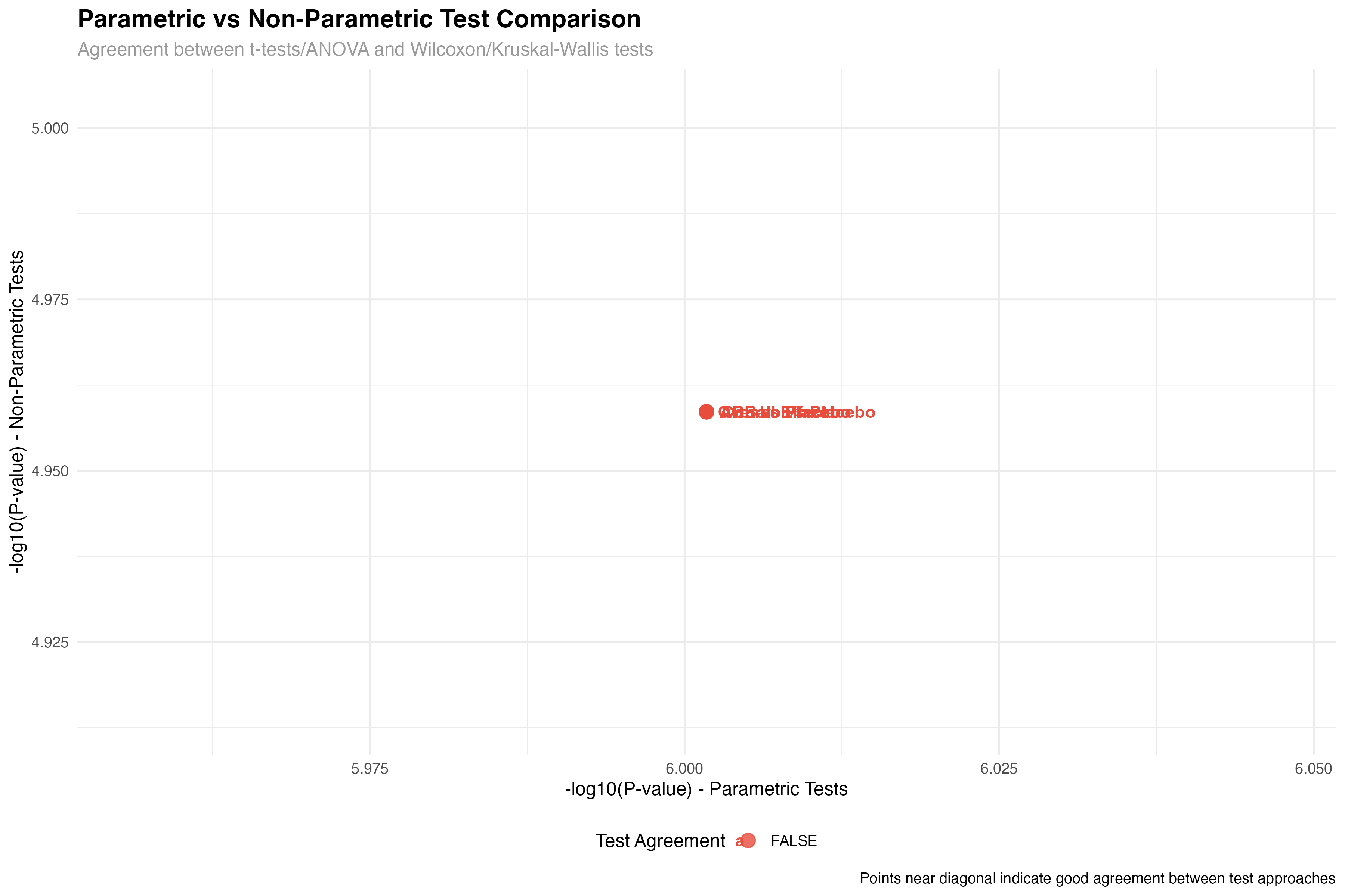
# Decision tree for test selection
test_selection <- normality_tests %>%
mutate(
normality_ok = p > 0.05,
recommended_test = case_when(
normality_ok ~ "Parametric (t-test/ANOVA)",
!normality_ok ~ "Non-parametric (Wilcoxon/Kruskal-Wallis)"
)
)
Correlation Analysis and Relationships
Understanding variable relationships with rstatix
# Correlation matrix with rstatix
cor_matrix <- primary_analysis_data %>%
  select(sbp, dbp, quality_of_life, age, bmi, baseline_sbp, baseline_dbp) %>%
  cor_mat()

# Correlation tests with p-values
cor_tests <- primary_analysis_data %>%
  cor_test(sbp, dbp, quality_of_life, age, bmi, method = "pearson")

# Partial correlation controlling for baseline
partial_cor <- primary_analysis_data %>%
  partial_cor_test(sbp, dbp, quality_of_life,
                   controlling.for = c("baseline_sbp", "baseline_dbp"))

# Display significant correlations
significant_correlations <- cor_tests %>%
  filter(p < 0.05) %>%
  arrange(p) %>%
  mutate(
    correlation_strength = case_when(
      abs(cor) >= 0.7 ~ "Strong",
      abs(cor) >= 0.4 ~ "Moderate",
      abs(cor) >= 0.2 ~ "Weak",
      TRUE ~ "Negligible"
    )
  )

print(significant_correlations)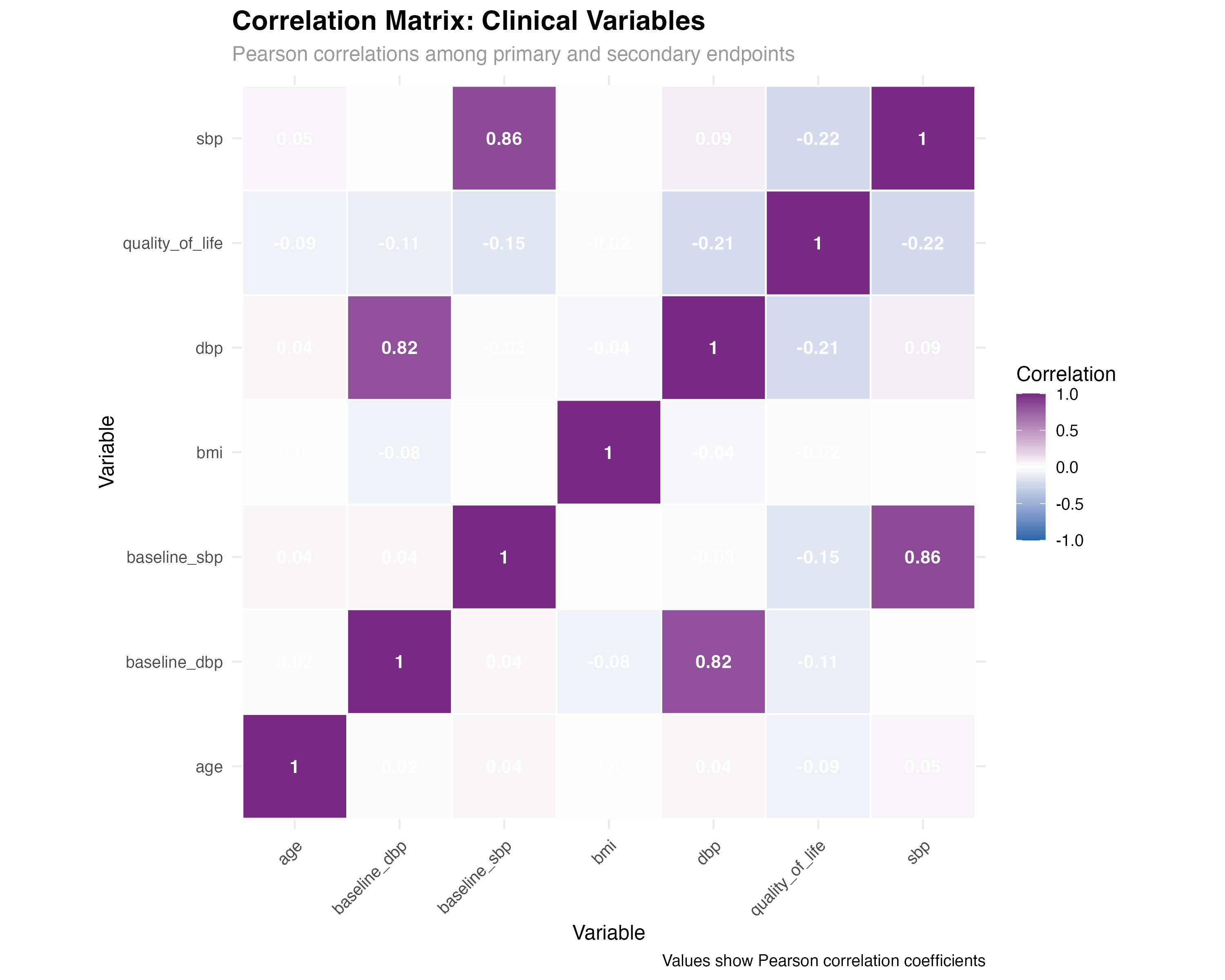
🔍 Correlation Insights
rstatix correlation analysis reveals clinically meaningful relationships: Strong BP correlations support using composite endpoints; Baseline-outcome correlations justify covariate adjustment; QoL-BP relationships validate patient-reported outcomes. The cor_test() function provides both effect sizes and statistical significance, enabling comprehensive relationship assessment.
Comprehensive Analysis Dashboard
Integrated rstatix workflow results
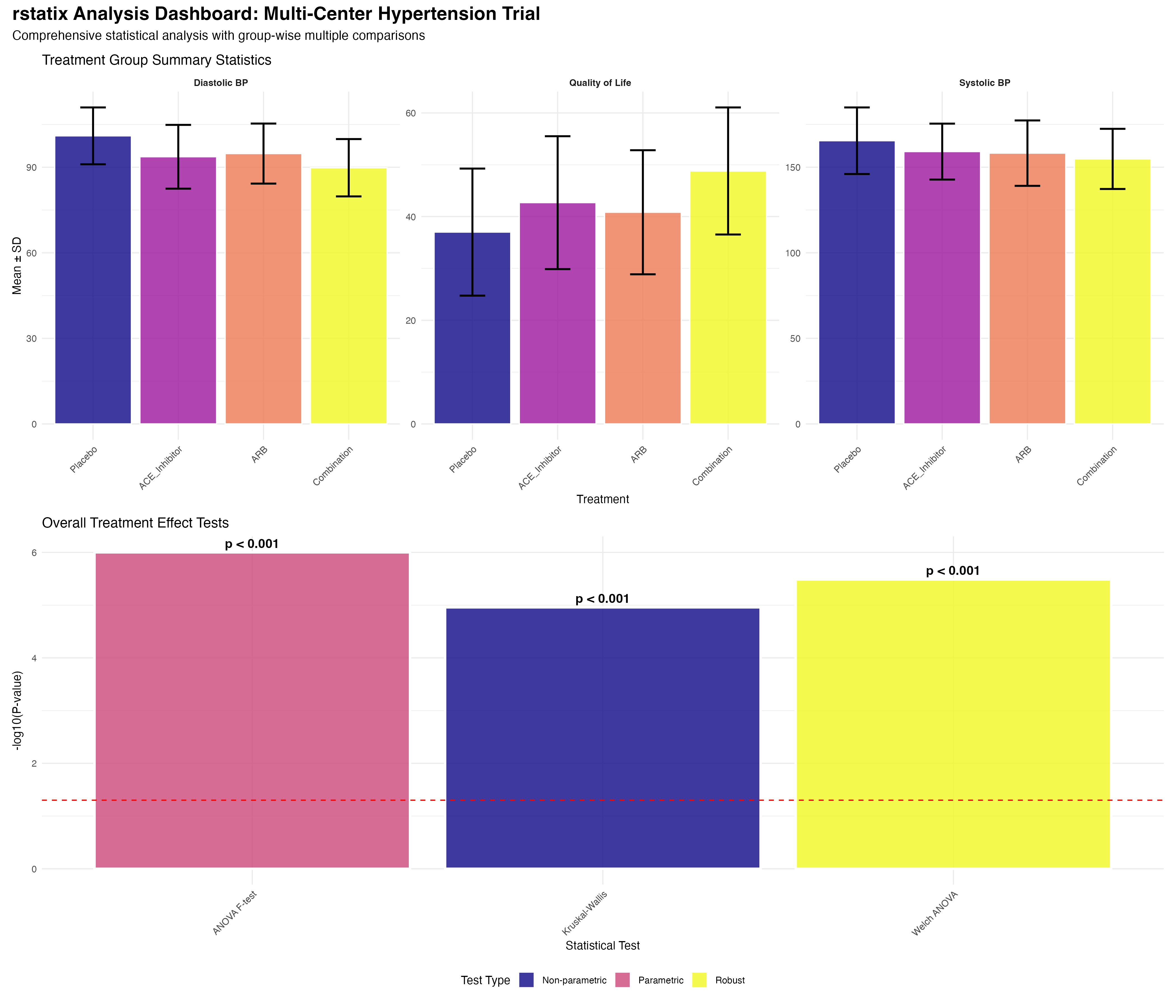
Used get_summary_stats() for comprehensive descriptive statistics by treatment groups and subgroups. Created age categories and risk stratification for group-wise analysis.
Applied shapiro_test() for normality assessment across groups. Used Q-Q plots for visual confirmation. Selected appropriate parametric vs non-parametric approaches.
Conducted anova_test() for overall treatment effects. Calculated effect sizes and confidence intervals. Applied multiple comparison corrections systematically.
Leveraged group_by() workflows for center-specific, age group, and risk category analyses. Applied appropriate correction methods for each analysis level.
Calculated cohens_d() for standardized effect sizes. Interpreted clinical meaningfulness beyond statistical significance. Provided context for clinical decision-making.
Integrated ggpubr for automated statistical annotations. Created publication-ready figures with p-values and effect sizes. Generated comprehensive analysis dashboard.
🔑 Key rstatix Advantages
Best Practices and Recommendations
Implementing rstatix in clinical research workflows